Can Solidworks Handle Hanging Chains?

Short answer: kind of, but it's not ideal and probably not worth it.

Background: Who cares about hanging chains?

Most people involved in creating gridshell structures care about hanging chains! They care because of the unique shape that a hanging chain makes - it is called a catenary, and it is important structurally because it represents a system in pure tension. This makes sense logically, because the chain is being pulled down by gravity at all points. This can be proven using calculus (infinite sum of small masses being pulled by gravity and by its neighbors - sounds like a FEA problem!), but its application greatly exceeds its creation.

Hanging chain

Uses of Catenary Shapes

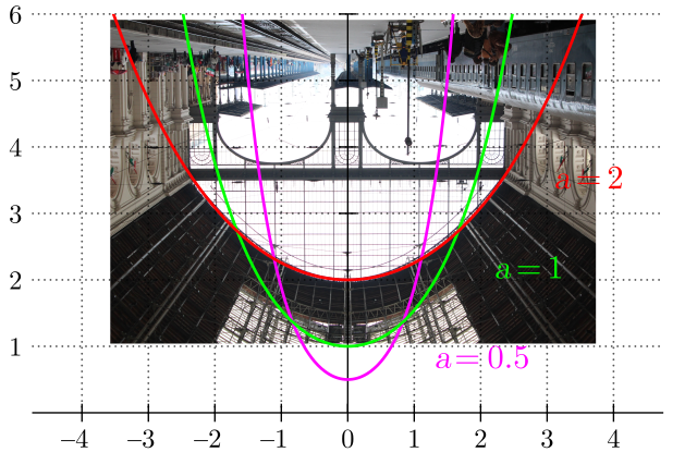
Catenary shapes are hanging systems in pure tension - but what would happen if you flipped one? Well, the chain would fall down and make another catenary. Now what if you solidify the chain, and then flip it? The result is a unique arch shape that is ideally in pure compression. This is used in architecture, such as the Keleti Railway Station in Budpaest, Hungary. When the upright photo is inverted and placed against a graph of a catenary curve, it matches very well, suggesting that the arch is indeed a catenary arch:

Keleti Station in Budpaest, Hungary

Keleti Station in Budpaest, Hungary

These catenary shapes can be applied to gridshell structures, essentially created from a lattice of hanging chains, that are then flipped and become the form of the gridshell structure.

Why Solidworks?

Solidworks has a Finite Element Analysis plugin, which we will be investigating to determine if it is robust enough for the research. We already know that Solidworks should be able to handle making a 3D model of a gridshell structure, and we know the simulation package can handle dynamic loads, which will be necessary for this research.

The first part of creating a hanging chain is designing and modeling a chain link; one that can be replicated and link into each other. Once the link is finished, the next step was to create a part to hold the hanging chain, so that the simulation can keep the holder fixed and apply a gravitational force to the chain links, creating the catenary shape. The chain link and chain holder part are:

Chain Link

Chain Holder

Once the parts were created, they were combined into an assembly. After the chain link was created (setting the number of links to adjust how far down the chain will hang), a Basic Motion Study was created, and gravitational force was added. When the motion study was run, the program produced a five-second video of the chain bouncing around, and when the video ended, the chain was hanging in what I presume to be a catenary shape, as shown below.

Oblique view of hanging chain

Heads-on view of hanging chain

Conclusion: Solidworks is Probably not the King of Catenaries

Solidworks was in fact able to handle a hanging chain, but there are a few limitations that probably sound the death knoll for Solidworks as a tool to decide the ideal shape for a gridshell. The first is the labor involved in creating the assembly. First, you have to create the chain link and the chain holder, then manually attach every chain link to each other. This would be prohibitively labor intensive for a longer chain, or a network of chains. Also, the computational resources involved in simulating even this basic chain were enough to strain my school laptop. 

And even if doing a more complex hanging chain was feasible, it is still not clear whether it is possible to export the locations of the chain links, in order to make a model of the chain link. If it turns out to be possible to get some sort of printout of the chain link positions, I could spline along the points and create a curve, along which I could sweep a cross-section, thus creating an arch (or a network of arches to make a gridshell).

How Would You (mostly) Automate a FEA Problem in MATLAB?

In order to make a MATLAB program to (mostly) automate solving a Finite Element Analysis problem, all you have to do is follow the same steps in the previous post. In summary:

1. Define Element Type
2. Define Node Positions/Representations
3. Define Nodal Connections (i.e. members)
4. Setup Local Matrices
5. Determine Positions in Global Matrix
6. Insert Local Matrices into Global Matrix
7. Determine Constraints and Trim Global Matrix Accordingly
8. Apply Forces, and Solve

For this exercise, I solved the example from the last post, which also allowed me to compare the results between the book, the hand calculations, and my Matlab program. The code is commented and clearly shows each step:

Note: If the formatted version is too hard to read, skip to the bottom for the plain text version copied directly from Matlab

FEM Example 2.1

% Sam Ciocco
clear, clc, close all;

Variable Inputs

numElements = 6; %Number of elements
numNodes = 5; %Number of nodes

DOF = 2; %Degrees of Freedom

A = 8; %Area in in^2
E = 1.9E6; %Elastic Modulus, in lb/in^2

forces = [0;0;0;0;0;0;0;-500;0;-500]; %Forces Vector, in order 1x;1y;2x;2y;...

constrained = [1,3]; %List of constrained nodes

Element Table

% For now, going to hardcode the table
% Will add node locations to calculate lengths and angles if I have time

elements = ones(numElements,7);
for i=1:numElements
    elements(i,1) = i;
end

% Declare the first node for each element
elements(:,2) = [1;2;3;2;2;4];
% Declare the second node for each element
elements(:,3) = [2;3;4;4;5;5];
% Declare lengths for each element
elements(:,4) = [36;50.9;36;36;50.9;36];
% Declare angles for each element, in degrees
elements(:,5) = [0;135;0;90;45;0];

%Insert sine and cosine for each element, based on the angle
for j=1:numElements
    elements(j,6) = cosd(elements(j,5));
    elements(j,7) = sind(elements(j,5));
end

%Element table organized as follows:
% Element | Node 1 | Node 2 | Length (in) | Angle (deg) | Cosine | Sine

Set up each local matrix

%Apparently I figured out how to make an array of matrices
for i=1:numElements
    keq(i) = A*E/elements(i,4);
    Klocal(:,:,i) = keq(i).*[elements(i,6)^2,elements(i,6)*elements(i,7),-(elements(i,6)^2),-elements(i,6)*elements(i,7);
                elements(i,6)*elements(i,7),elements(i,7)^2,-elements(i,6)*elements(i,7),-(elements(i,7)^2);
                -(elements(i,6)^2),-elements(i,6)*elements(i,7),elements(i,6)^2,elements(i,6)*elements(i,7);
                -elements(i,6)*elements(i,7),-(elements(i,7)^2),elements(i,6)*elements(i,7),elements(i,7)^2];
end

Set up Global Matrix

% Declare a matrix of correct size for each node to have its number of
% degrees of freedom (DOF)

Kglobal = zeros(numNodes*DOF,numNodes*DOF);

% Now painstakingly fill in each local matrix into the global matrix
% Ensuring each local matrix is placed correctly according to its nodes
for i=1:numElements
    for j=0:1
       for k=0:1
           Kglobal(elements(i,2)*2-1+j,elements(i,2)*2-1+k) = Kglobal(elements(i,2)*2-1+j,elements(i,2)*2-1+k)+Klocal(j+1,k+1,i);
       end
    end

    for j=0:1
       for k=0:1
           Kglobal(elements(i,2)*2-1+j,elements(i,3)*2-1+k) = Kglobal(elements(i,3)*2-1+j,elements(i,2)*2-1+k)+Klocal(j+1,k+3,i);
       end
    end

    for j=0:1
       for k=0:1
           Kglobal(elements(i,3)*2-1+j,elements(i,3)*2-1+k) = Kglobal(elements(i,3)*2-1+j,elements(i,3)*2-1+k)+Klocal(j+3,k+3,i);
       end
    end

    for j=0:1
       for k=0:1
           Kglobal(elements(i,3)*2-1+j,elements(i,2)*2-1+k) = Kglobal(elements(i,3)*2-1+j,elements(i,2)*2-1+k)+Klocal(j+3,k+1,i);
       end
    end

    % Old code, not completely sure why it didn't work

%     Kglobal(elements(i,2)*2-1,elements(i,2)*2-1) = Kglobal(elements(i,2)*2-1,elements(i,2)*2-1)+Klocal(1,1,i);
%     Kglobal(elements(i,2)*2-1,elements(i,2)*2-1+1) = Kglobal(elements(i,2)*2-1,elements(i,2)*2-1+1)+Klocal(1,2,i);
%     Kglobal(elements(i,2)*2-1+1,elements(i,2)*2-1) = Kglobal(elements(i,2)*2-1+1,elements(i,2)*2-1)+Klocal(2,1,i);
%     Kglobal(elements(i,2)*2-1+1,elements(i,2)*2-1+1) = Kglobal(elements(i,2)*2-1+1,elements(i,2)*2-1+1)+Klocal(2,2,i);
end

Create list of unconstrained (aka moving) nodes

    % This code assumes each node can either move or not; no partial
    % constraints

nodes = 1:numNodes; %Create list of nodes
movingNum = 1;
moving = zeros(numNodes-length(constrained));
for i=1:numNodes
        if((nodes(i) ~= constrained(1)) && (nodes(i) ~= constrained(2)))
            moving(movingNum) = i;
            movingNum = movingNum+1;
        end
end

Trim Global Matrix in Accordance with Constrained Nodes

% Again assuming any constrained nodes are fully constrained

Kglobal2 = zeros((numNodes-length(constrained))*2,(numNodes-length(constrained))*2);

    for i=1:length(moving)
        for j=1:length(moving)

            for k=0:1
                for m=0:1

                    Kglobal2(i*2-1+k,j*2-1+m) = Kglobal(moving(i)*2-1+k,moving(j)*2-1+m);


                end
            end
        end
    end

% for l=1:length(moving)
% for i=:1
%     for j=0:1
%     Kglobal2(l*2-1+i,l*2-1+j) = Kglobal(moving(l)*2-1+i,moving(l)*2-1+j);
%
%     end
% end
% end

Trim Forces in Accordance with Constrained Nodes

forces2 = zeros(length(moving)*2,1);

for l=1:length(moving)
    forces2(l*2-1) = forces(moving(l)*2-1);
    forces2(l*2) = forces(moving(l)*2);
end

Solve Matrix for movements

movements = Kglobal2\forces2;
%movements is the vector of the first node x, the first node y, the second
%node x, the second node y,...


numMoving = 1;
for i=1:2:length(movements)

            fprintf('\nThe movement of node %.0f in the x-direction is %.3f inches\n',moving(numMoving),movements(i));
            fprintf('The movement of node %.0f in the y-direction is %.3f inches\n',moving(numMoving),movements(i+1));
            numMoving = numMoving+1;

end

The movement of node 2 in the x-direction is -0.004 inches
The movement of node 2 in the y-direction is -0.010 inches

The movement of node 4 in the x-direction is 0.001 inches
The movement of node 4 in the y-direction is -0.011 inches

The movement of node 5 in the x-direction is 0.002 inches
The movement of node 5 in the y-direction is -0.020 inches

Published with MATLAB® R2015a

Plain Text Version:

%% FEM Example 2.1

% Sam Ciocco

clear, clc, close all;

%% Variable Inputs

numElements = 6; %Number of elements

numNodes = 5; %Number of nodes

DOF = 2; %Degrees of Freedom

A = 8; %Area in in^2

E = 1.9E6; %Elastic Modulus, in lb/in^2

forces = [0;0;0;0;0;0;0;-500;0;-500]; %Forces Vector, in order 1x;1y;2x;2y;...

constrained = [1,3]; %List of constrained nodes

%% Element Table

% For now, going to hardcode the table

% Will add node locations to calculate lengths and angles if I have time

elements = ones(numElements,7);

for i=1:numElements

    elements(i,1) = i;

end

% Declare the first node for each element

elements(:,2) = [1;2;3;2;2;4];

% Declare the second node for each element

elements(:,3) = [2;3;4;4;5;5];

% Declare lengths for each element

elements(:,4) = [36;50.9;36;36;50.9;36];

% Declare angles for each element, in degrees

elements(:,5) = [0;135;0;90;45;0];

%Insert sine and cosine for each element, based on the angle

for j=1:numElements

    elements(j,6) = cosd(elements(j,5));

    elements(j,7) = sind(elements(j,5));

end

%Element table organized as follows:

% Element | Node 1 | Node 2 | Length (in) | Angle (deg) | Cosine | Sine

%% Set up each local matrix

%Apparently I figured out how to make an array of matrices

for i=1:numElements

    keq(i) = A*E/elements(i,4);

    Klocal(:,:,i) = keq(i).*[elements(i,6)^2,elements(i,6)*elements(i,7),-(elements(i,6)^2),-elements(i,6)*elements(i,7);

                elements(i,6)*elements(i,7),elements(i,7)^2,-elements(i,6)*elements(i,7),-(elements(i,7)^2);

                -(elements(i,6)^2),-elements(i,6)*elements(i,7),elements(i,6)^2,elements(i,6)*elements(i,7);

                -elements(i,6)*elements(i,7),-(elements(i,7)^2),elements(i,6)*elements(i,7),elements(i,7)^2];

end

%% Set up Global Matrix

% Declare a matrix of correct size for each node to have its number of

% degrees of freedom (DOF)

Kglobal = zeros(numNodes*DOF,numNodes*DOF);

% Now painstakingly fill in each local matrix into the global matrix

% Ensuring each local matrix is placed correctly according to its nodes

for i=1:numElements

    for j=0:1

       for k=0:1

           Kglobal(elements(i,2)*2-1+j,elements(i,2)*2-1+k) = Kglobal(elements(i,2)*2-1+j,elements(i,2)*2-1+k)+Klocal(j+1,k+1,i);

       end

    end

    

    for j=0:1

       for k=0:1

           Kglobal(elements(i,2)*2-1+j,elements(i,3)*2-1+k) = Kglobal(elements(i,3)*2-1+j,elements(i,2)*2-1+k)+Klocal(j+1,k+3,i);

       end

    end

    

    for j=0:1

       for k=0:1

           Kglobal(elements(i,3)*2-1+j,elements(i,3)*2-1+k) = Kglobal(elements(i,3)*2-1+j,elements(i,3)*2-1+k)+Klocal(j+3,k+3,i);

       end

    end

    

    for j=0:1

       for k=0:1

           Kglobal(elements(i,3)*2-1+j,elements(i,2)*2-1+k) = Kglobal(elements(i,3)*2-1+j,elements(i,2)*2-1+k)+Klocal(j+3,k+1,i);

       end

    end

    

    % Old code, not completely sure why it didn't work

    

%     Kglobal(elements(i,2)*2-1,elements(i,2)*2-1) = Kglobal(elements(i,2)*2-1,elements(i,2)*2-1)+Klocal(1,1,i);

%     Kglobal(elements(i,2)*2-1,elements(i,2)*2-1+1) = Kglobal(elements(i,2)*2-1,elements(i,2)*2-1+1)+Klocal(1,2,i);

%     Kglobal(elements(i,2)*2-1+1,elements(i,2)*2-1) = Kglobal(elements(i,2)*2-1+1,elements(i,2)*2-1)+Klocal(2,1,i);

%     Kglobal(elements(i,2)*2-1+1,elements(i,2)*2-1+1) = Kglobal(elements(i,2)*2-1+1,elements(i,2)*2-1+1)+Klocal(2,2,i);

end

    

%% Create list of unconstrained (aka moving) nodes

    % This code assumes each node can either move or not; no partial

    % constraints

    

nodes = 1:numNodes; %Create list of nodes

movingNum = 1;

moving = zeros(numNodes-length(constrained));

for i=1:numNodes

        if((nodes(i) ~= constrained(1)) && (nodes(i) ~= constrained(2)))

            moving(movingNum) = i;

            movingNum = movingNum+1;

        end

end

%% Trim Global Matrix in Accordance with Constrained Nodes

% Again assuming any constrained nodes are fully constrained

Kglobal2 = zeros((numNodes-length(constrained))*2,(numNodes-length(constrained))*2);

    for i=1:length(moving)

        for j=1:length(moving)

        

            for k=0:1

                for m=0:1

        

                    Kglobal2(i*2-1+k,j*2-1+m) = Kglobal(moving(i)*2-1+k,moving(j)*2-1+m);

        

        

                end

            end

        end

    end

% for l=1:length(moving)

% for i=:1

%     for j=0:1

%     Kglobal2(l*2-1+i,l*2-1+j) = Kglobal(moving(l)*2-1+i,moving(l)*2-1+j);

%     

%     end

% end

% end

%% Trim Forces in Accordance with Constrained Nodes

forces2 = zeros(length(moving)*2,1);

for l=1:length(moving)

    forces2(l*2-1) = forces(moving(l)*2-1);

    forces2(l*2) = forces(moving(l)*2);

end

%% Solve Matrix for movements

movements = Kglobal2\forces2;

%movements is the vector of the first node x, the first node y, the second

%node x, the second node y,...

numMoving = 1;

for i=1:2:length(movements)

    

            fprintf('\nThe movement of node %.0f in the x-direction is %.3f inches\n',moving(numMoving),movements(i));

            fprintf('The movement of node %.0f in the y-direction is %.3f inches\n',moving(numMoving),movements(i+1));

            numMoving = numMoving+1;

            

end

Starting with the Basics: How does Finite Element Analysis Work?

What Even Is 'Finite Element Analysis'?

Finite Element Analysis is the process by which an engineering problem can be modeled as the sum of multiple smaller, simpler problems. For example, a 2-D truss problem can be modeled with each two-force member acting as a simple spring. The creation of this model is referred to as Finite Element Modeling. The use of Finite Element Modeling allows complex problems to be solved numerically through the use of matrices, in the process known as Finite Element Analysis.

How Do You Set up a Finite Element Model?

The basic steps to setting up any finite element model, for any system (though it is easiest to think of a problem in terms of a physical system) is as follows:

1. Define Element Type - in the example above, a truss element may treat every member as simple springs, whereas a beam may treat each member as having 2 full dimensions of space. This determines where each member will be, and where each node will be (members connect two or more nodes).
2. Define Node Positions/Representations - In a physical system, a node is usually a junction of two members, but could connect more, or could be an intermediate point somewhere along a member. For a system representing heat transfer or something else, a node could be a point at which a material property can be measured or calculated.
3. Define Nodal Connections (i.e. members) - Members connect the nodes, and each member must be defined as connecting its nodes, because that member then represents the force between the two nodes.
4. Setup Local Matrices - Each member has a local matrix that contains the definition for which nodes that member connects, and the stiffness (or corresponding material property) is a measure of how rigidly the member connects the nodes.
5. Determine Local Positions in Global Matrix - Each local matrix will fit into one larger global matrix, that contains the relationships between every node to every other node.
6. Insert Local Matrices into Global Matrix - every local matrix must be slotted into its position in the global matrix before the problem can be solved. If multiple elements contain relationships for the same node, they are added or subtracted accordingly to obtain the final, inclusive set of nodal relationships.
7. Determine Constrains and Trim Global Matrix Accordingly - Constraints are sometimes necessary for solving a problem in that they reduce the number of unknowns by declaring that certain nodes will behave in certain ways (i.e. node 1 is fixed, node 2 can move in X but not Y, etc). These constraints allow the global matrix to be trimmed, resulting in a smaller final computation and a less resource-intensive solution.
8. Apply Forces, and Solve - Finite Element Analysis problems are solved in the formula of Global*Resultant = Forces, where the Global and Forces matrices have already been trimmed to match the forced sections of the Resultant matrix. The problem can be solved numerically by hand or by a computer, handheld or otherwise.

Can you solve an FEM problem by hand?

Yes, you can! In fact, I did. Here's the work, numbered after the fact, following the steps outlined above:

One thing to note is that the top table contains a few extra calculations, namely the sine, cosine, and length of each member, to be readily accessible later. Also, the number 7 refers to the X's marked across the global matrix, which show the rows and columns that represent the constrained nodes.

The Resultant matrix is defined as a vector of deflection variables, which are given as an output of solving the system of matrices, shown in the box on the right of the second page.