Semester Goal for This Research

What is the End of the Semester Goal for this Research?

At the end of the semester, this research needs to yield a paper, a presentation, and a poster. That means that at some point, my advisor and I need to figure out exactly what we want to get out of this project. This will have to be dialed in precisely over the next few weeks, but here is what we have so far:

Strain Energy Convergence

When running a finite element analysis for a given model under a given load, the strain energy is the sum of the strain in every element. A finer mesh means the model will have more elements, and for a coarse mesh range, more elements will mean a higher total strain energy. Eventually, the model will have enough elements to accurately represent the strain in the model, and a finer mesh will not increase the strain energy anymore. This is called strain energy convergence, and ideally it should resemble a horizontal asymptote.

This is the graph from testing the 10x10 spherical cap (the model will be explained later in this post):

Total Strain Energy vs. 1/Mesh Length for 10x20 spherical cap

The graph doesn't quite reach convergence, but given the limitations of the technology at hand, it is going to have to be close enough (and it is reasonably close, we aren't even going to use the finest mesh shown).

Running a model with finer meshes until strain energy convergence gives the coarsest mesh that still shows all the strain in the model. In simpler terms, it shows the least process-intensive model to still get accurate results. In this case, it is somewhere around 0.08-0.05m, and most likely we will use 0.08m because that can run on my Naval Academy issued laptop.

What models are going to be run at this mesh?

This semester's research will most likely focus on rigid models instead of pre-tensioned models for sake of simplicity. This will allow us to evaluate multiple models (pre-tensioning just takes too long to create multiple models of the same form) and evaluate them under different member spacings and cross-sections to examine structural differences from having different numbers of members.

To show this process, I will be making three rigid gridshell models, all spherical caps with perpendicular members; one will have 10x10 members, then 20x20, and finally a 30x30 model. All three models are the same overall size, and for now they have the same cross section:

10x10 Spherical Cap Rigid Model

20x20 Spherical Cap Rigid Model

30x30 Spherical Cap Rigid Model (unfinished)

Why have Three Different Models?

The models will all be evaluated under the mesh size found from the strain energy convergence of the 10x10 (we will run strain energy convergence tests on the others to make sure 0.08m works for all three). These models will be compared on the basis of volume/mass (given a material), buckling load, and probably maximum stress/deflection given a prescribed load. Another interesting option may be to prescribe a load case and a maximum allowable stress, and then find the necessary cross section for each model to meet that criteria.

This comparison will explore the inherent trade-offs of changing member spacing. The next post will hopefully contain more specifics of the end-of-semester deliverables of this research.

Form-Finding

What is Form-Finding?

Form-finding is  the way in which computer programs easily simulate the hanging-spring networks mentioned previously in this blog. Form-finding fits into the larger algorithm of this research:

1. Set 2-D grid

2. Use form-finding to optimize the grid for a given height

3. Convert the simple, shell model into distinct members

4. Create members in Solidworks and mark/note their intersection points

5. Create Solidworks assembly of grid of members

6. Add connections to members

7. Erect the gridshell assembly

8. Test the gridshell in Solidworks Simulation

Steps 3-8 of the process come from the work I did at my internship, which in turn come from the process in which real gridshells are constructed: you lay the members flat on the ground, attach the joints, then raise the gridshell and lock it into place. Steps 1 and 2 are the new part.

Why use form-finding at all?

During the internship, the shape of the gridshell was determined by my Matlab code; its dimensions didn't need to have any basis in reality. That is not the case under the new system, in which the research is set up to directly complement the gridshell capstone project here at the Academy.

What does form-finding have to do with capstone?

My capstone project is to design a gridshell that can essentially compete with a standardized SWA hut for Humanitarian Assidance/Disaster Relief (HA/DR) applications. This means that at some point, the capstone group will have to pick a size and rough shape of the capstone (in order to solidify materials needed, weight, interior space, etc). Once this happens, or even to help this happen, I can use form-finding to test any size gridshell that the capstone group needs.

PushMePullMe

PushMePullMe, which will now be referred to as PMPM, is a form-finding function that works well for gridshells, as shown by the model below, which took all of ten minutes to make:

Basic gridshell model found using PushMePullMe 3-D

PMPM, as far as I've found, isn't terribly precise in its height criteria for optimization, but it is extremely quick to raise the gridshell optimally once the grid and anchors are laid out on the ground.

We will also be looking into using Rhino with the Grasshopper plugin to allow for more precise parametric design in the optimization, but I haven't had a chance to look at that yet.

Taking a form from a shell model to Solidworks

A model such as the above PMPM model isn't exactly correct as far as the members; in the model above, all the members are on the same shell, which means they all take up no space and go through each other. Real gridshells have stacked members sandwiched with plates, which need to be modeled to ensure an accurate result.

Going from points generated from a model such as the above, and creating a Solidworks sketch is a fairly simple process, using one macro found online:

Simple Solidworks sketch from points

This model, however, still has all the members on the same plane, and wouldn't allow for the stacked members. This means I must manipulate the points in order to get one member at a time. Then I need the length of that member so that I can lay it flat in Solidworks and then get the pre-tension when the gridshell is raised.

I have done this before, over the internshp. Here is the Matlab plot of the points used to make the above sketch (note that the axes aren't the same scale so the cap dome looks much higher than it really is):

Matlab plot of points used to make Solidworks sketch shown above

By looking through the coordinate arrays, I was able to isolate one cross-member. This allowed me to then spline the points of that beam to create close to a smooth curve. This almost-smooth curve then allows me to measure and output the length of the member and the length in between intersection points, which I need in order to lay the flat grid of members in Solidworks. The plot below shows the nodes and spline of one member:

2-D Plot of one member in Matlab.

The blue circles are the nodes that define the member, and the red curve is the points that make up the spline approximation for the shape of the member, allowing me to calculate its overall length and length between nodes.

Next Steps

The next thing to try will be Rhino with Grasshopper. I am confident that I could finish the spherical cap, as it would essentially be the same process used in the last part of the internship. Focusing on steps 1 and 2 will also allow the research to better integrate with the capstone project.

Pre-Tension in a Gridshell

How would you model pre-tension in a gridshell caused by bending members in Solidworks?

Apparently, Solidworks has the capability to model the pre-tension, by essentially replicating the bending process, which allows the user to start with this model;

Gridshell Beam Model

And bend it a prescribed amount, resulting in this:

Bent Gridshell Beam

It is worth noting that, while this beam is correctly matched to the height and length of a gridshell (calculated mathematically in Matlab), it is only constrained via prescribed displacement at the ends, but the capability exists to constrain several points along the beam, ensuring the final shape matches the desired catenary curve.

Now, can this method handle bolted connections?

Turns out Solidworks also does that pretty well. I started the test with a simple cross of two long beams, connected with the standard curved plate and bolt connection used previously. The result (note this one uses several prescribed displacements to ensure a slightly more accurate catenary shape) is shown below:

Basic Bolted Joint Bent

Which also started laid out flat:

Basic Bolted Joint Model

This model involved most of the same process as before:

1. Lay out the members flat
2. Use Assembly mates to achieve the desired position and layout
3. Fix the center of each beam (this leaves both plates able to flex)
4. Sketch lines into the beams to create the edges that will have prescribed deflections
5. Prescribe the deflections, making use of the "Split" option for selecting lines partway down the beam

Now, what if the bolted connection moves?

The next logical step was to see what happens if the bolted connection itself needs to move with the beam; how will Solidworks handle having the bolted connections moving like that? Will everything stay together as it should, or will the bolts do something unrealistic?

To test this, I started making a simple 5-member gridshell, in the shape of a catenary dome, as shown below modeled in Matlab:

Matlab 3-D Plot of 5-Member Catenary Dome

I haven't yet added all the members, but here is the flat assembly so far:

Unfinished Catenary Gridshell Laid Flat

It's hard to see, but each point where beams cross has a full bolted connection (bolted between two curved plates, that might have to change eventually to a more simple shape). The end of each beam was constrained to drop 2m vertically, so that everything ends up at "ground" level. The resulting model doesn't really look like a catenary shape (the next step is to use the Matlab model and constrain each joint to drop by the correct amount), but it shows that the bolted connections managed to hold up, even when the whole joint moves:

Unfinished Catenary Gridshell Bent

The next step is to add more complexity to this model to make it actually resemble the Matlab plot. In order to make the model match the plot, a few things must be added:

1. Add the other cross-beams, with 6 more bolted plate connections
2. Constrain each connection to displace its correct amount
3. If that still doesn't accurately resemble a catenary dome, then move on to prescribing the displacement of each beam at a few intermediate points

Working with Simulation in Solidworks

How do you make sure a bolted connection will model correctly in Solidworks?

Here are a few realizations I had about making sure a simulation of a bolted connection will run correctly:

1. Friction - Solidworks Help page says that friction is added automatically based on the materials chosen, but it isn't (note there is nowhere in material properties to add a coefficient of friction; it's based on both materials contacting, not just one). This means that every component contact must have a coefficient of friction set; if this varies, then multiple component contacts will be needed to fully define the model
2. Solver - The Solver matters; different solvers are better at different things. Most notably, the Direct Sparse Solver, while being potentially less accurate than the Iterative Solver, can better make use of powerful multi-threaded CPU's (such as the 32-thread Xeon in the Watkins Hall computer lab)

Solving With 'FFEPlus' Iterative Solver - Note 3% overall usage and one core used

Solving with 'Intel Direct Sparse' - Note 39% overall usage and most cores used

3. Washers on Bolted Connections - Washers are commonly used on bolted connections to avoid preload loss at the head or nut of a bolt due to deformation when the contact stress deforms the material where the head/nut presses. However, after reading about their use in bolted connections in Solidworks, I don't think it is necessary to add washers in the simulation, and it has the tendency to make the simulation not actually solve. It seems best, then, to leave washers out (maybe adjust the radius of the head and/or nut, I'm not sure how that works, I'm going to check that out next).

Update: Bolt head size does work in Solidworks Simulation

After testing the same model with a larger bolt head, it would seem Solidworks does in fact model the size of the bolt head (why would they let the user define the bolt head/nut size if they didn't?). This means that the user can use a larger bolt head to model a washer of the same size. Proof shown below:

Joint Model with 12mm Bolt Head - Note the lighter sections (more stress) around the bolt 

Identical Joint Model with 20mm Bolt Head - Note the area around the bolt is now light blue - lower contact stress

Bolted Connections In Solidworks - Gridshell Joint Exercise

Can Solidworks easily handle a bolted connection?

Or: Practice Working on a Gridshell Joint

Gridshells are generally laid out on the ground, then propped into their final shape by scaffolding (or other means, as will be the subject of next year's capstone project). This means that a gridshell joint needs to be attached on the ground while still allowing rotational and longitudinal freedom of its members, and then locked into place when the final form is attained.

The most common way this is achieved today is through the use of clamped plates that sandwich the gridshell members. They are initially applied loosely to allow the members to flex and slide during the erection of the gridshell, and then clamped more tightly later to lock the gridshell into the correct form.

Modeling this joint in Solidworks is a hurdle this research will eventually have to face, due to the potential effect the joints will have on the structure that cannot be modeled by a simple rigid connection. But doing this in Solidworks requires using a bolted connection, which the author was not sure if Solidworks actually had the capability to handle natively. It turns out Solidworks does have this ability, and it really isn't too terribly hard.

In a Solidworks Simulation (in this case a static simulation set to study the stresses on the clamping plates due to rotating force in the members), the user simply needs to select the drop-down menu under 'Connections Advisor' and select 'Bolt' and follow the setup to select the cylindrical cuts the bolt will go through, and the ends where the head and nut will be. This selection even allows for a set preload, a crucial part of any bolted connection (a preload applies the clamping force and prevents joint separation, allowing the joint to be treated as one rigid member).

Approximation of a Gridshell Joint, Showing Bolted Connections

A real clamped connection on a Gridshell would have additional complexity, such as plate shapes that are more visually appealing, and washers (and even some disk springs) on the bolted connection, that are not modeled here. These can be added later to this model or a new model if this ends up being too far from reality.

With that disclaimer in mind, it was possible to run this model, which yielded the following stress visualization:

Approximation of a Gridshell Joint, Under a Twisting Force on the 'Gridshell Members'

This shows almost no load on the members themselves, and almost all of the load on the plates. While this may or may not resemble a realistic connection (ideally the members should only be transmitting compression forces, as shown in the last post), it does show that the bolts are transmitting load through the clamping force they exert.

I also found out that Solidworks does in fact have a way to treat a member as a beam (including selecting joints), so the next step will be to check that out, and see if it is feasible for use in this project.

Testing Catenary Arch and Catenary Dome

How do you verify that a shape is a catenary?

A catenary shape is defined as the shape a hanging chain makes, resulting in pure tension. When flipped, the resulting catenary arch should, under equal and opposite gravitational load, be in a state of pure compression.

To verify the catenary shapes that I made in Solidworks, I turned them into a catenary arch and a catenary dome, using the following procedure:

1. Create a sketch of the center of each 'node' in the hanging chain model
2. Copy the sketch into a new Solidworks part file
3. Spline the points together
4. Sweep a cross section along the spline
5. Fix the ends of the arch/corners of the dome
6. Apply gravitational load
7. View results, if the compression load is close to equal throughout the part, then it can be considered a catenary arch/dome

Using the spline took to create a continuous curve and sweeping the cross section along the curve yielded the following parts:

Catenary Arch

Catenary Dome

With the ends of the arch and corners of the dome fixed and gravitational load applied, the stress visualization showed that the parts are indeed approximately catenary shapes (Note that it was easier to flip the gravitational force than it would have been to flip the part):

Catenary Arch Under Graviational Load

Catenary Dome Under Graviational Load

The side view shows that the shapes (except for near the fixtures, especially on the arch) have a consistent stress throughout the part, further proving that they are roughly catenary shapes:

Catenary Arch Under Gravitational Load, Side View

Catenary Dome Under Gravitational Load, Side View

This means that using Solidworks to model a hanging chain could, indeed, be used as a tool for generating catenary curves to be used in gridshell design. Another option I have been pursuing is using Matlab to create a catenary equation for a given size and shape (input desired height and width, and the script solves for the necessary curvature, and outputs the list of points for the desired shape/form)

Hanging Grid of Spring Chains

Can Solidworks Handle a Matrix of Hanging Spring Chains?

Yes, with similar procedure as the catenary shape of the chain of springs, only this time there is a grid (or matrix) or springs, making a 'catenary dome' that could eventually be used to make a gridshell. The result ends up looking as expected:

Spring Chain Matrix, Hanging

Just as with a single spring chain, starting from a flat position ensures that the hanging is repeatable, and the curvature of the form (basically how far down the chains actually hang) can be manipulated by adjusting the spring constant of the springs, either individually or together.

Spring Chain Matrix Starting Position (disregard the red springs)

Adjusting the springs individually will change the shape from a standard catenary shape, however, and would only make sense when the flipped catenary dome will be under uneven loading.

Both the single spring chain and the spring chain matrix were able to yield sketches representing the position of each 'node,' which means the next step moving forward is to turn those sketches into an actual catenary arch (and eventually a catenary dome) and test them under even graviational loading to see if they are at or near pure compression.

Hanging Spring Chains with Solidworks

Why Include Springs in a Hanging Chain?

Real chains, like all materials, have some springiness associated with them, as defined by their coefficient of elasticity (also known as Young's Modulus). As shown earlier in the post about what FEM is, a spring with it's spring constant (k) can accurately model a material with it's modulus of elasticity (E).

When modeling a rigid chain, the only way to adjust how far the chain sags is to add or remove links to change the length of the chain itself. This changing mechanic is limited by the length of each change, as the chain has to have a whole number of links added or removed. A spring chain, however, can adjust the spring constant of each link to manipulate how far down the chain hangs, allowing for much finer adjustments. Every time a spring chain is hung, it can be reset to the same level starting position, making the experiment repeatable:

Spring Chain Model, Starting Position

And will end in a catenary curve, defined by the total length of the span and the spring constant:

Spring Chain Model, Catenary Curve

The number of links, in this case, serves more to make a cleaner curve than to change its shape, with more links making a smoother curve, because each spring is assumed to be linear by itself. Each connection between the springs is simply a small cylinder, that is assumed to be a point. The mass of each member can possibly be changed to change the gravitational force, but the shape will most likely only be changed by manipulating the spring constant.

The next step is to read more about Solidworks' Motion Study, to find if/how the motion can be exported, preferably as a text file of element positions, so that I can turn that back into a curve shape to model and test. If I can get points that make the catenary curve, I can import the points back into Solidworks, then spline along the curve, then sweep a cross section along the curve, creating one catenary arch. This process, if possible, can be expanded across a network of springs to create a complete gridshell shape.

Can Solidworks Handle Hanging Chains?

Short answer: kind of, but it's not ideal and probably not worth it.

Background: Who cares about hanging chains?

Most people involved in creating gridshell structures care about hanging chains! They care because of the unique shape that a hanging chain makes - it is called a catenary, and it is important structurally because it represents a system in pure tension. This makes sense logically, because the chain is being pulled down by gravity at all points. This can be proven using calculus (infinite sum of small masses being pulled by gravity and by its neighbors - sounds like a FEA problem!), but its application greatly exceeds its creation.

Hanging chain

Uses of Catenary Shapes

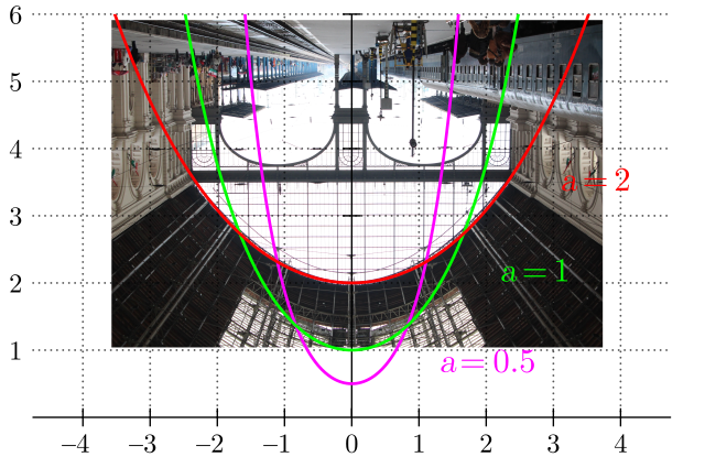
Catenary shapes are hanging systems in pure tension - but what would happen if you flipped one? Well, the chain would fall down and make another catenary. Now what if you solidify the chain, and then flip it? The result is a unique arch shape that is ideally in pure compression. This is used in architecture, such as the Keleti Railway Station in Budpaest, Hungary. When the upright photo is inverted and placed against a graph of a catenary curve, it matches very well, suggesting that the arch is indeed a catenary arch:

Keleti Station in Budpaest, Hungary

Keleti Station in Budpaest, Hungary

These catenary shapes can be applied to gridshell structures, essentially created from a lattice of hanging chains, that are then flipped and become the form of the gridshell structure.

Why Solidworks?

Solidworks has a Finite Element Analysis plugin, which we will be investigating to determine if it is robust enough for the research. We already know that Solidworks should be able to handle making a 3D model of a gridshell structure, and we know the simulation package can handle dynamic loads, which will be necessary for this research.

The first part of creating a hanging chain is designing and modeling a chain link; one that can be replicated and link into each other. Once the link is finished, the next step was to create a part to hold the hanging chain, so that the simulation can keep the holder fixed and apply a gravitational force to the chain links, creating the catenary shape. The chain link and chain holder part are:

Chain Link

Chain Holder

Once the parts were created, they were combined into an assembly. After the chain link was created (setting the number of links to adjust how far down the chain will hang), a Basic Motion Study was created, and gravitational force was added. When the motion study was run, the program produced a five-second video of the chain bouncing around, and when the video ended, the chain was hanging in what I presume to be a catenary shape, as shown below.

Oblique view of hanging chain

Heads-on view of hanging chain

Conclusion: Solidworks is Probably not the King of Catenaries

Solidworks was in fact able to handle a hanging chain, but there are a few limitations that probably sound the death knoll for Solidworks as a tool to decide the ideal shape for a gridshell. The first is the labor involved in creating the assembly. First, you have to create the chain link and the chain holder, then manually attach every chain link to each other. This would be prohibitively labor intensive for a longer chain, or a network of chains. Also, the computational resources involved in simulating even this basic chain were enough to strain my school laptop. 

And even if doing a more complex hanging chain was feasible, it is still not clear whether it is possible to export the locations of the chain links, in order to make a model of the chain link. If it turns out to be possible to get some sort of printout of the chain link positions, I could spline along the points and create a curve, along which I could sweep a cross-section, thus creating an arch (or a network of arches to make a gridshell).

How Would You (mostly) Automate a FEA Problem in MATLAB?

In order to make a MATLAB program to (mostly) automate solving a Finite Element Analysis problem, all you have to do is follow the same steps in the previous post. In summary:

1. Define Element Type
2. Define Node Positions/Representations
3. Define Nodal Connections (i.e. members)
4. Setup Local Matrices
5. Determine Positions in Global Matrix
6. Insert Local Matrices into Global Matrix
7. Determine Constraints and Trim Global Matrix Accordingly
8. Apply Forces, and Solve

For this exercise, I solved the example from the last post, which also allowed me to compare the results between the book, the hand calculations, and my Matlab program. The code is commented and clearly shows each step:

Note: If the formatted version is too hard to read, skip to the bottom for the plain text version copied directly from Matlab

FEM Example 2.1

% Sam Ciocco
clear, clc, close all;

Variable Inputs

numElements = 6; %Number of elements
numNodes = 5; %Number of nodes

DOF = 2; %Degrees of Freedom

A = 8; %Area in in^2
E = 1.9E6; %Elastic Modulus, in lb/in^2

forces = [0;0;0;0;0;0;0;-500;0;-500]; %Forces Vector, in order 1x;1y;2x;2y;...

constrained = [1,3]; %List of constrained nodes

Element Table

% For now, going to hardcode the table
% Will add node locations to calculate lengths and angles if I have time

elements = ones(numElements,7);
for i=1:numElements
    elements(i,1) = i;
end

% Declare the first node for each element
elements(:,2) = [1;2;3;2;2;4];
% Declare the second node for each element
elements(:,3) = [2;3;4;4;5;5];
% Declare lengths for each element
elements(:,4) = [36;50.9;36;36;50.9;36];
% Declare angles for each element, in degrees
elements(:,5) = [0;135;0;90;45;0];

%Insert sine and cosine for each element, based on the angle
for j=1:numElements
    elements(j,6) = cosd(elements(j,5));
    elements(j,7) = sind(elements(j,5));
end

%Element table organized as follows:
% Element | Node 1 | Node 2 | Length (in) | Angle (deg) | Cosine | Sine

Set up each local matrix

%Apparently I figured out how to make an array of matrices
for i=1:numElements
    keq(i) = A*E/elements(i,4);
    Klocal(:,:,i) = keq(i).*[elements(i,6)^2,elements(i,6)*elements(i,7),-(elements(i,6)^2),-elements(i,6)*elements(i,7);
                elements(i,6)*elements(i,7),elements(i,7)^2,-elements(i,6)*elements(i,7),-(elements(i,7)^2);
                -(elements(i,6)^2),-elements(i,6)*elements(i,7),elements(i,6)^2,elements(i,6)*elements(i,7);
                -elements(i,6)*elements(i,7),-(elements(i,7)^2),elements(i,6)*elements(i,7),elements(i,7)^2];
end

Set up Global Matrix

% Declare a matrix of correct size for each node to have its number of
% degrees of freedom (DOF)

Kglobal = zeros(numNodes*DOF,numNodes*DOF);

% Now painstakingly fill in each local matrix into the global matrix
% Ensuring each local matrix is placed correctly according to its nodes
for i=1:numElements
    for j=0:1
       for k=0:1
           Kglobal(elements(i,2)*2-1+j,elements(i,2)*2-1+k) = Kglobal(elements(i,2)*2-1+j,elements(i,2)*2-1+k)+Klocal(j+1,k+1,i);
       end
    end

    for j=0:1
       for k=0:1
           Kglobal(elements(i,2)*2-1+j,elements(i,3)*2-1+k) = Kglobal(elements(i,3)*2-1+j,elements(i,2)*2-1+k)+Klocal(j+1,k+3,i);
       end
    end

    for j=0:1
       for k=0:1
           Kglobal(elements(i,3)*2-1+j,elements(i,3)*2-1+k) = Kglobal(elements(i,3)*2-1+j,elements(i,3)*2-1+k)+Klocal(j+3,k+3,i);
       end
    end

    for j=0:1
       for k=0:1
           Kglobal(elements(i,3)*2-1+j,elements(i,2)*2-1+k) = Kglobal(elements(i,3)*2-1+j,elements(i,2)*2-1+k)+Klocal(j+3,k+1,i);
       end
    end

    % Old code, not completely sure why it didn't work

%     Kglobal(elements(i,2)*2-1,elements(i,2)*2-1) = Kglobal(elements(i,2)*2-1,elements(i,2)*2-1)+Klocal(1,1,i);
%     Kglobal(elements(i,2)*2-1,elements(i,2)*2-1+1) = Kglobal(elements(i,2)*2-1,elements(i,2)*2-1+1)+Klocal(1,2,i);
%     Kglobal(elements(i,2)*2-1+1,elements(i,2)*2-1) = Kglobal(elements(i,2)*2-1+1,elements(i,2)*2-1)+Klocal(2,1,i);
%     Kglobal(elements(i,2)*2-1+1,elements(i,2)*2-1+1) = Kglobal(elements(i,2)*2-1+1,elements(i,2)*2-1+1)+Klocal(2,2,i);
end

Create list of unconstrained (aka moving) nodes

    % This code assumes each node can either move or not; no partial
    % constraints

nodes = 1:numNodes; %Create list of nodes
movingNum = 1;
moving = zeros(numNodes-length(constrained));
for i=1:numNodes
        if((nodes(i) ~= constrained(1)) && (nodes(i) ~= constrained(2)))
            moving(movingNum) = i;
            movingNum = movingNum+1;
        end
end

Trim Global Matrix in Accordance with Constrained Nodes

% Again assuming any constrained nodes are fully constrained

Kglobal2 = zeros((numNodes-length(constrained))*2,(numNodes-length(constrained))*2);

    for i=1:length(moving)
        for j=1:length(moving)

            for k=0:1
                for m=0:1

                    Kglobal2(i*2-1+k,j*2-1+m) = Kglobal(moving(i)*2-1+k,moving(j)*2-1+m);


                end
            end
        end
    end

% for l=1:length(moving)
% for i=:1
%     for j=0:1
%     Kglobal2(l*2-1+i,l*2-1+j) = Kglobal(moving(l)*2-1+i,moving(l)*2-1+j);
%
%     end
% end
% end

Trim Forces in Accordance with Constrained Nodes

forces2 = zeros(length(moving)*2,1);

for l=1:length(moving)
    forces2(l*2-1) = forces(moving(l)*2-1);
    forces2(l*2) = forces(moving(l)*2);
end

Solve Matrix for movements

movements = Kglobal2\forces2;
%movements is the vector of the first node x, the first node y, the second
%node x, the second node y,...


numMoving = 1;
for i=1:2:length(movements)

            fprintf('\nThe movement of node %.0f in the x-direction is %.3f inches\n',moving(numMoving),movements(i));
            fprintf('The movement of node %.0f in the y-direction is %.3f inches\n',moving(numMoving),movements(i+1));
            numMoving = numMoving+1;

end

The movement of node 2 in the x-direction is -0.004 inches
The movement of node 2 in the y-direction is -0.010 inches

The movement of node 4 in the x-direction is 0.001 inches
The movement of node 4 in the y-direction is -0.011 inches

The movement of node 5 in the x-direction is 0.002 inches
The movement of node 5 in the y-direction is -0.020 inches

Published with MATLAB® R2015a

Plain Text Version:

%% FEM Example 2.1

% Sam Ciocco

clear, clc, close all;

%% Variable Inputs

numElements = 6; %Number of elements

numNodes = 5; %Number of nodes

DOF = 2; %Degrees of Freedom

A = 8; %Area in in^2

E = 1.9E6; %Elastic Modulus, in lb/in^2

forces = [0;0;0;0;0;0;0;-500;0;-500]; %Forces Vector, in order 1x;1y;2x;2y;...

constrained = [1,3]; %List of constrained nodes

%% Element Table

% For now, going to hardcode the table

% Will add node locations to calculate lengths and angles if I have time

elements = ones(numElements,7);

for i=1:numElements

    elements(i,1) = i;

end

% Declare the first node for each element

elements(:,2) = [1;2;3;2;2;4];

% Declare the second node for each element

elements(:,3) = [2;3;4;4;5;5];

% Declare lengths for each element

elements(:,4) = [36;50.9;36;36;50.9;36];

% Declare angles for each element, in degrees

elements(:,5) = [0;135;0;90;45;0];

%Insert sine and cosine for each element, based on the angle

for j=1:numElements

    elements(j,6) = cosd(elements(j,5));

    elements(j,7) = sind(elements(j,5));

end

%Element table organized as follows:

% Element | Node 1 | Node 2 | Length (in) | Angle (deg) | Cosine | Sine

%% Set up each local matrix

%Apparently I figured out how to make an array of matrices

for i=1:numElements

    keq(i) = A*E/elements(i,4);

    Klocal(:,:,i) = keq(i).*[elements(i,6)^2,elements(i,6)*elements(i,7),-(elements(i,6)^2),-elements(i,6)*elements(i,7);

                elements(i,6)*elements(i,7),elements(i,7)^2,-elements(i,6)*elements(i,7),-(elements(i,7)^2);

                -(elements(i,6)^2),-elements(i,6)*elements(i,7),elements(i,6)^2,elements(i,6)*elements(i,7);

                -elements(i,6)*elements(i,7),-(elements(i,7)^2),elements(i,6)*elements(i,7),elements(i,7)^2];

end

%% Set up Global Matrix

% Declare a matrix of correct size for each node to have its number of

% degrees of freedom (DOF)

Kglobal = zeros(numNodes*DOF,numNodes*DOF);

% Now painstakingly fill in each local matrix into the global matrix

% Ensuring each local matrix is placed correctly according to its nodes

for i=1:numElements

    for j=0:1

       for k=0:1

           Kglobal(elements(i,2)*2-1+j,elements(i,2)*2-1+k) = Kglobal(elements(i,2)*2-1+j,elements(i,2)*2-1+k)+Klocal(j+1,k+1,i);

       end

    end

    

    for j=0:1

       for k=0:1

           Kglobal(elements(i,2)*2-1+j,elements(i,3)*2-1+k) = Kglobal(elements(i,3)*2-1+j,elements(i,2)*2-1+k)+Klocal(j+1,k+3,i);

       end

    end

    

    for j=0:1

       for k=0:1

           Kglobal(elements(i,3)*2-1+j,elements(i,3)*2-1+k) = Kglobal(elements(i,3)*2-1+j,elements(i,3)*2-1+k)+Klocal(j+3,k+3,i);

       end

    end

    

    for j=0:1

       for k=0:1

           Kglobal(elements(i,3)*2-1+j,elements(i,2)*2-1+k) = Kglobal(elements(i,3)*2-1+j,elements(i,2)*2-1+k)+Klocal(j+3,k+1,i);

       end

    end

    

    % Old code, not completely sure why it didn't work

    

%     Kglobal(elements(i,2)*2-1,elements(i,2)*2-1) = Kglobal(elements(i,2)*2-1,elements(i,2)*2-1)+Klocal(1,1,i);

%     Kglobal(elements(i,2)*2-1,elements(i,2)*2-1+1) = Kglobal(elements(i,2)*2-1,elements(i,2)*2-1+1)+Klocal(1,2,i);

%     Kglobal(elements(i,2)*2-1+1,elements(i,2)*2-1) = Kglobal(elements(i,2)*2-1+1,elements(i,2)*2-1)+Klocal(2,1,i);

%     Kglobal(elements(i,2)*2-1+1,elements(i,2)*2-1+1) = Kglobal(elements(i,2)*2-1+1,elements(i,2)*2-1+1)+Klocal(2,2,i);

end

    

%% Create list of unconstrained (aka moving) nodes

    % This code assumes each node can either move or not; no partial

    % constraints

    

nodes = 1:numNodes; %Create list of nodes

movingNum = 1;

moving = zeros(numNodes-length(constrained));

for i=1:numNodes

        if((nodes(i) ~= constrained(1)) && (nodes(i) ~= constrained(2)))

            moving(movingNum) = i;

            movingNum = movingNum+1;

        end

end

%% Trim Global Matrix in Accordance with Constrained Nodes

% Again assuming any constrained nodes are fully constrained

Kglobal2 = zeros((numNodes-length(constrained))*2,(numNodes-length(constrained))*2);

    for i=1:length(moving)

        for j=1:length(moving)

        

            for k=0:1

                for m=0:1

        

                    Kglobal2(i*2-1+k,j*2-1+m) = Kglobal(moving(i)*2-1+k,moving(j)*2-1+m);

        

        

                end

            end

        end

    end

% for l=1:length(moving)

% for i=:1

%     for j=0:1

%     Kglobal2(l*2-1+i,l*2-1+j) = Kglobal(moving(l)*2-1+i,moving(l)*2-1+j);

%     

%     end

% end

% end

%% Trim Forces in Accordance with Constrained Nodes

forces2 = zeros(length(moving)*2,1);

for l=1:length(moving)

    forces2(l*2-1) = forces(moving(l)*2-1);

    forces2(l*2) = forces(moving(l)*2);

end

%% Solve Matrix for movements

movements = Kglobal2\forces2;

%movements is the vector of the first node x, the first node y, the second

%node x, the second node y,...

numMoving = 1;

for i=1:2:length(movements)

    

            fprintf('\nThe movement of node %.0f in the x-direction is %.3f inches\n',moving(numMoving),movements(i));

            fprintf('The movement of node %.0f in the y-direction is %.3f inches\n',moving(numMoving),movements(i+1));

            numMoving = numMoving+1;

            

end

Starting with the Basics: How does Finite Element Analysis Work?

What Even Is 'Finite Element Analysis'?

Finite Element Analysis is the process by which an engineering problem can be modeled as the sum of multiple smaller, simpler problems. For example, a 2-D truss problem can be modeled with each two-force member acting as a simple spring. The creation of this model is referred to as Finite Element Modeling. The use of Finite Element Modeling allows complex problems to be solved numerically through the use of matrices, in the process known as Finite Element Analysis.

How Do You Set up a Finite Element Model?

The basic steps to setting up any finite element model, for any system (though it is easiest to think of a problem in terms of a physical system) is as follows:

1. Define Element Type - in the example above, a truss element may treat every member as simple springs, whereas a beam may treat each member as having 2 full dimensions of space. This determines where each member will be, and where each node will be (members connect two or more nodes).
2. Define Node Positions/Representations - In a physical system, a node is usually a junction of two members, but could connect more, or could be an intermediate point somewhere along a member. For a system representing heat transfer or something else, a node could be a point at which a material property can be measured or calculated.
3. Define Nodal Connections (i.e. members) - Members connect the nodes, and each member must be defined as connecting its nodes, because that member then represents the force between the two nodes.
4. Setup Local Matrices - Each member has a local matrix that contains the definition for which nodes that member connects, and the stiffness (or corresponding material property) is a measure of how rigidly the member connects the nodes.
5. Determine Local Positions in Global Matrix - Each local matrix will fit into one larger global matrix, that contains the relationships between every node to every other node.
6. Insert Local Matrices into Global Matrix - every local matrix must be slotted into its position in the global matrix before the problem can be solved. If multiple elements contain relationships for the same node, they are added or subtracted accordingly to obtain the final, inclusive set of nodal relationships.
7. Determine Constrains and Trim Global Matrix Accordingly - Constraints are sometimes necessary for solving a problem in that they reduce the number of unknowns by declaring that certain nodes will behave in certain ways (i.e. node 1 is fixed, node 2 can move in X but not Y, etc). These constraints allow the global matrix to be trimmed, resulting in a smaller final computation and a less resource-intensive solution.
8. Apply Forces, and Solve - Finite Element Analysis problems are solved in the formula of Global*Resultant = Forces, where the Global and Forces matrices have already been trimmed to match the forced sections of the Resultant matrix. The problem can be solved numerically by hand or by a computer, handheld or otherwise.

Can you solve an FEM problem by hand?

Yes, you can! In fact, I did. Here's the work, numbered after the fact, following the steps outlined above:

One thing to note is that the top table contains a few extra calculations, namely the sine, cosine, and length of each member, to be readily accessible later. Also, the number 7 refers to the X's marked across the global matrix, which show the rows and columns that represent the constrained nodes.

The Resultant matrix is defined as a vector of deflection variables, which are given as an output of solving the system of matrices, shown in the box on the right of the second page.